Gradient Descent for linear regression task Data pre processing
Load data from csv file to a list
1
2
3
4
5
trainDataList = list () with open ("train.csv" , newline="" ) as csvfile: trainData = csv.reader(csvfile, delimiter="," ,quotechar="|" ) for line in trainData: trainDataList.append(line[3 :])
make all train data in one list, to enable iterating per hour of the list, thus, we have (24 * days - 10 + 1) training data.
trainDataIteratedPerHour: list()
1 2 3 4 5 6 7 8 9 10 11 12 13 14 15 16 17 18 19 20 21 22 23 24 25 26 27 28 29 30 31 32 33 def mod_18 (n ): return n % 18 def T_list (l ): return np.array(l).T.tolist() i = 0 trainDataIteratedPerHour = [] listToAppend = [] for item in trainDataList[1 :]: if not mod_18(i): listToAppend = [item] elif mod_18(i) == 10 : listToAppend.append(["0" if x == 'NR' else x for x in item]) elif mod_18(i) == 17 : listToAppend.append(item) trainDataIteratedPerHour.extend(T_list(listToAppend)) else : listToAppend.append(item) i = i + 1 i = 0
1
2
3
4
5
6
7
8
9
10
11
12
13
14
""" build x_data and y_data """ x_data = [] y_data = [] for n in range (len (trainDataIteratedPerHour) - 10 ): x_data.extend(np.array(trainDataIteratedPerHour[n : n + 9 ]).reshape(1 ,162 ).tolist()) y_data.append(trainDataIteratedPerHour[n + 10 ][9 ]) x_data = [[float (j) for j in i] for i in x_data] y_data = [float (i) for i in y_data]
draw plot (to feel the range of the data)
1 2 3 4 5 6 7 8 9 10 11 12 13 import matplotlibimport matplotlib.pyplot as pltx = range (len (y_data)) y = np.array(y_data) fig, ax = plt.subplots() ax.plot(x, y)
Loss function 1 2 3 4 5 6 7 8 9 10 11 12 def lossFunction (w, x_data, y_data ): w = np.array(w) x_data = np.array(x_data) result = 0. for i in range (len (y_data)): result += (y_data[i] - sum (w * x_data[i]))**2 return result
Iterations for grident descent 1 2 3 4 5 6 7 8 9 10 11 12 13 14 15 16 17 18 19 20 21 22 23 24 25 26 27 def iterationRun (lr,iteration,x_data,y_data ): w = [0.01 ] * 162 L_history = [lossFunction(w,x_data,y_data)] w = np.array(w) x_data = np.array(x_data) for iterator in range (iteration): w_grad = [0.0 ] * 162 for n in range (len (y_data)): for i in range (162 ): w_grad[i] = w_grad[i] - 2.0 * x_data[n][i] * ( sum (w * x_data[n]) - y_data[n] ) for i in range (162 ): w[i] = w[i] + lr * w_grad[i] L_history.append(lossFunction(w,x_data,y_data)) print (str (iterator) + " : " + str (datetime.datetime.now().time()) + " L:" + str (L_history[-1 ])) return L_history
Run it for 10 iterations
1 2 3 lr = 0.0000000000001 iteration = 10 iterationRun(lr,iteration,x_data,y_data)
Tunning Find good initial learning rate start with lr = 0.0000000000001
1 2 3 4 5 6 7 8 9 10 In [19 ]: lr = 0.0000000000001 ...: iteration = 10 ...: iterationRun(lr,iteration,x_data,y_data) ...: 0 : 13 :21 :22.227145 L:5897161.869645979 1 : 13 :21 :53.988814 L:5890818.193569232 2 : 13 :22 :25.639150 L:5884483.073933817 3 : 13 :22 :57.211950 L:5878156.49918669 4 : 13 :23 :28.873442 L:5871838.457790465 5 : 13 :24 :01.059230 L:5865528.93822318
hmmm… try greater lr
lr = 0.00000000001
The loss function is descenting faster, like around 60000 per epoch.
1 2 3 4 5 6 7 8 9 10 11 12 13 In [21 ]: lr = 0.000000000001 ...: iteration = 10 ...: iterationRun(lr,iteration,x_data,y_data) ...: 0 : 13 :35 :09.910428 L:5840184.58334736 1 : 13 :35 :41.650901 L:5777706.652466557 2 : 13 :36 :13.323090 L:5716068.8576254565 3 : 13 :36 :45.001751 L:5655259.889673614 4 : 13 :37 :16.168479 L:5595268.591697776 5 : 13 :37 :47.701241 L:5536083.956972405 6 : 13 :38 :19.216952 L:5477695.126938047 7 : 13 :38 :51.013157 L:5420091.389206737
our training set data is 5750
1 2 In [20 ]: len (y_data) Out[20 ]: 5750
If prediected pm 2.5 value , a.k.a y data is in error range 10, the L value should be 5750*100=575000
With current descent speed, we will need 88 epoch:
1 2 In [24 ]: (5840184 -575000 )/60000 Out[24 ]: 87.75306666666667
let’s make it 10 times faster to see if target L could be get in 10 epoch
lr = 0.0000000001
1 2 3 4 5 6 7 8 9 10 11 12 13 14 15 16 17 18 19 20 21 22 23 24 25 26 In [27 ]: lr = 0.0000000001 ...: iteration = 10 ...: iterationRun(lr,iteration,x_data,y_data) ...: 0 : 13 :49 :10.609660 L:1692576.375268496 1 : 13 :49 :42.475991 L:1242849.9101765472 2 : 13 :50 :14.660518 L:1189717.4416525147 3 : 13 :50 :46.605178 L:1178550.5080278912 4 : 13 :51 :18.416010 L:1171963.6339294983 5 : 13 :51 :50.342550 L:1166008.2433918654 6 : 13 :52 :22.022203 L:1160260.444018784 7 : 13 :52 :53.942997 L:1154668.3447938378 8 : 13 :53 :25.925997 L:1149219.7383900573 9 : 13 :53 :57.718994 L:1143907.0426408767 Out[27 ]: [5903514.1137326835 , 1692576.375268496 , 1242849.9101765472 , 1189717.4416525147 , 1178550.5080278912 , 1171963.6339294983 , 1166008.2433918654 , 1160260.444018784 , 1154668.3447938378 , 1149219.7383900573 , 1143907.0426408767 ]
1 2 3 4 5 6 7 x = range (iteration+1 ) y = np.array(L_history) fig, ax = plt.subplots() ax.plot(x, y)
As we printed in first step only, we can see now the learning rate is way faster in initial step thus the first L printed is in smaller range!
And we also know it’s descenting slower after 10 ephoch, thus it’s not reaching our target 575000 in small steps.
I (for sure) know that I need to use adaptive learning rate and customised learning rate per feature(adagrade/ adam), while before that, I would like to see how it goes with smaller learning rate, while it goes to mess!
1 2 3 4 5 6 7 8 In [46 ]: lr = 0.000000001 ...: iteration = 10 ...: iterationRun(lr,iteration,x_data,y_data) ...: 0 : 14 :09:17.516243 L:156704618.55348668 1 : 14 :09:49.509213 L:5150723049.19715 2 : 14 :10 :21.436315 L:170469039390.23218 3 : 14 :10 :53.396840 L:5642995478812.637
lr = 1e-10 Then we could back to last initial learning rate, let’s get the final w by adding print (w) in iterationRun() , also we add initial w as an argument to enable modified initial w
1 2 3 4 5 6 7 8 9 10 11 12 13 14 15 16 17 18 19 20 21 22 23 24 25 26 def iterationRun (lr,iteration,x_data,y_data, w = [0.01 ] * 162 ): L_history = [lossFunction(w,x_data,y_data)] w = np.array(w) x_data = np.array(x_data) for iterator in range (iteration): w_grad = [0.0 ] * 162 for n in range (len (y_data)): for i in range (162 ): w_grad[i] = w_grad[i] - 2.0 * x_data[n][i] * ( sum (w * x_data[n]) - y_data[n] ) for i in range (162 ): w[i] = w[i] + lr * w_grad[i] L_history.append(lossFunction(w,x_data,y_data)) print (str (iterator) + " : " + str (datetime.datetime.now().time()) + " L:" + str (L_history[-1 ])) print (w) return L_history
Then after re-run, we got the w:
1 2 3 4 5 6 7 8 9 10 11 12 13 14 15 16 17 18 19 20 21 22 23 24 25 26 27 28 29 30 31 32 33 34 35 36 37 38 39 40 41 42 43 44 45 46 47 48 49 50 51 52 53 In [49 ]: lr = 0.0000000001 ...: iteration = 10 ...: iterationRun(lr,iteration,x_data,y_data) ...: 0 : 14 :24 :45.664141 L:1692576.375268496 1 : 14 :25 :17.259352 L:1242849.9101765472 2 : 14 :25 :49.273630 L:1189717.4416525147 3 : 14 :26 :20.965149 L:1178550.5080278912 4 : 14 :26 :52.781849 L:1171963.6339294983 5 : 14 :27 :24.309887 L:1166008.2433918654 6 : 14 :27 :56.071350 L:1160260.444018784 7 : 14 :28 :27.729255 L:1154668.3447938378 8 : 14 :28 :59.185918 L:1149219.7383900573 9 : 14 :29 :31.678511 L:1143907.0426408767 [0.00865451 0.00992088 0.00998412 0.00999356 0.00989859 0.00958899 0.00949017 0.00853832 0.00886119 0.00971015 0.00996496 0.00622562 0.00986532 0.00991454 0.00047019 0.0002918 0.00985504 0.009888 0.00866327 0.00992104 0.00998492 0.00999403 0.00990841 0.00960856 0.00951873 0.00854217 0.00888944 0.00973543 0.00996355 0.00618855 0.00987026 0.00991514 0.00064165 0.00051266 0.00985705 0.00988871 0.00867558 0.00992112 0.00998615 0.00999456 0.00991583 0.00962887 0.00954697 0.00857636 0.00896101 0.00978193 0.00996072 0.00613156 0.00987708 0.0099157 0.00089779 0.00075592 0.00985905 0.00988954 0.00869251 0.0099212 0.00998776 0.00999517 0.009925 0.00965916 0.00958656 0.00863933 0.00905468 0.00984584 0.00995951 0.00605779 0.00988265 0.00991644 0.0011024 0.00105049 0.00986111 0.00989001 0.00871203 0.00992131 0.00998925 0.00999581 0.0099313 0.00969443 0.00962812 0.00874158 0.00919581 0.00993813 0.00996109 0.00597563 0.00989311 0.00991724 0.00152071 0.00139776 0.00986338 0.00989169 0.00873482 0.00992151 0.00999107 0.00999641 0.00993875 0.00973362 0.00967406 0.00888077 0.00938529 0.01006057 0.00996181 0.00589041 0.00990578 0.00991814 0.00187297 0.00190307 0.00986629 0.00989357 0.00875685 0.00992174 0.00999275 0.00999693 0.0099442 0.00977445 0.00972014 0.00904638 0.00964319 0.01023079 0.00996201 0.00581055 0.00992017 0.00991885 0.0023883 0.0023404 0.00986947 0.00989559 0.0087768 0.009922 0.00999477 0.00999745 0.00994748 0.00981834 0.0097673 0.00922359 0.00995879 0.01041849 0.00995968 0.00574316 0.00993535 0.00991957 0.00290124 0.00287465 0.00987295 0.0098975 0.00879132 0.0099223 0.00999638 0.00999786 0.00994411 0.00986186 0.0098075 0.00938749 0.0103109 0.0108169 0.00995914 0.00570475 0.00995173 0.00992029 0.0036527 0.00347423 0.00987645 0.00990038 ] Out[49 ]: [5903514.1137326835 , 1692576.375268496 , 1242849.9101765472 , 1189717.4416525147 , 1178550.5080278912 , 1171963.6339294983 , 1166008.2433918654 , 1160260.444018784 , 1154668.3447938378 , 1149219.7383900573 , 1143907.0426408767 ]
Run 10~20 epoch, lr=1e-10 Another 10 epoch( continued from first 10 epoch):
1 2 3 4 5 6 7 8 9 10 11 12 13 14 15 16 17 18 19 20 21 22 23 24 25 26 27 28 29 30 31 32 33 34 35 36 37 38 39 40 41 42 43 44 45 46 47 48 49 50 51 52 53 54 55 56 57 58 59 60 61 62 63 64 65 66 67 68 69 70 71 72 73 74 75 76 77 78 79 80 81 82 83 84 85 86 87 88 89 90 91 92 93 94 95 In [59 ]: lr = 0.0000000001 In [60 ]: iteration = 10 In [61 ]: iterationRun(lr,iteration,x_data,y_data,w) ...: 0 : 14 :41 :55.554137 L:1138723.54416636 1 : 14 :42 :27.844246 L:1133663.0986562215 2 : 14 :42 :59.894751 L:1128719.8759725974 3 : 14 :43 :32.401907 L:1123888.4508929225 4 : 14 :44 :04.728092 L:1119163.74563917 5 : 14 :44 :36.823878 L:1114541.0056141382 6 : 14 :45 :08.958169 L:1110015.776899496 7 : 14 :45 :41.079041 L:1105583.8853543748 8 : 14 :46 :13.182146 L:1101241.4171967693 9 : 14 :46 :45.360379 L:1096984.7009616988 [ 8.39928810e-03 9.92018594e-03 9.98672249e-03 9.99395695e-03 9.90650252e-03 9.66028161e-03 9.57133059e-03 8.59024624e-03 9.70063031e-03 1.04003048e-02 9.94007211e-03 5.82092975e-03 9.86818613e-03 9.91420797e-03 -7.30043313e-04 -9.74984684e-04 9.81897077e-03 9.85914945e-03 8.42038505e-03 9.92049552e-03 9.98824144e-03 9.99488279e-03 9.92479021e-03 9.70246400e-03 9.63010828e-03 8.61918398e-03 9.77660141e-03 1.04616680e-02 9.93740891e-03 5.73728090e-03 9.87953143e-03 9.91540645e-03 -2.36708203e-04 -4.46497772e-04 9.82369317e-03 9.86089703e-03 8.44699272e-03 9.92063613e-03 9.99060846e-03 9.99592360e-03 9.93769384e-03 9.74480356e-03 9.68631482e-03 8.69975569e-03 9.93568798e-03 1.05632875e-02 9.93195597e-03 5.62070493e-03 9.89358966e-03 9.91648735e-03 3.09727865e-04 3.32769386e-05 9.82806229e-03 9.86271172e-03 8.48109217e-03 9.92078753e-03 9.99374187e-03 9.99713322e-03 9.95409819e-03 9.80638186e-03 9.76454663e-03 8.82732248e-03 1.01321537e-02 1.06964648e-02 9.92985319e-03 5.47712005e-03 9.90438972e-03 9.91794789e-03 6.73973650e-04 5.44360035e-04 9.83218649e-03 9.86359313e-03 8.51878100e-03 9.92099916e-03 9.99667211e-03 9.99839142e-03 9.96501744e-03 9.87773770e-03 9.84678838e-03 9.02306858e-03 1.04158946e-02 1.08835903e-02 9.93324622e-03 5.32255768e-03 9.92446485e-03 9.91952209e-03 1.38594142e-03 1.10724366e-03 9.83633504e-03 9.86671984e-03 8.56162962e-03 9.92140609e-03 1.00002676e-02 9.99958471e-03 9.97874755e-03 9.95697261e-03 9.93834450e-03 9.28329913e-03 1.07901635e-02 1.11284264e-02 9.93483699e-03 5.16636435e-03 9.94860271e-03 9.92131553e-03 1.92598395e-03 1.94810223e-03 9.84148301e-03 9.87004892e-03 8.60192082e-03 9.92187479e-03 1.00036215e-02 1.00006191e-02 9.98884103e-03 1.00394245e-02 1.00304865e-02 9.58954906e-03 1.12961891e-02 1.14662940e-02 9.93528449e-03 5.02390839e-03 9.97597866e-03 9.92274238e-03 2.75467811e-03 2.63288432e-03 9.84692043e-03 9.87360657e-03 8.63756441e-03 9.92241075e-03 1.00076795e-02 1.00016598e-02 9.99478393e-03 1.01275708e-02 1.01245597e-02 9.91586834e-03 1.19162061e-02 1.18375866e-02 9.93069923e-03 4.90773511e-03 1.00047837e-02 9.92420129e-03 3.57134262e-03 3.51203380e-03 9.85289824e-03 9.87690267e-03 8.66241404e-03 9.92304041e-03 1.00109440e-02 1.00024858e-02 9.98759482e-03 1.02142033e-02 1.02041105e-02 1.02157481e-02 1.26087041e-02 1.26296733e-02 9.92961546e-03 4.84886429e-03 1.00360505e-02 9.92566063e-03 4.87428673e-03 4.54246885e-03 9.85895437e-03 9.88225200e-03 ] Out[61 ]: [1143907.0116957787 , 1138723.54416636 , 1133663.0986562215 , 1128719.8759725974 , 1123888.4508929225 , 1119163.74563917 , 1114541.0056141382 , 1110015.776899496 , 1105583.8853543748 , 1101241.4171967693 , 1096984.7009616988 ] In [62 ]: L_history = [1143907.0116957787 , ...: 1138723.54416636 , ...: 1133663.0986562215 , ...: 1128719.8759725974 , ...: 1123888.4508929225 , ...: 1119163.74563917 , ...: 1114541.0056141382 , ...: 1110015.776899496 , ...: 1105583.8853543748 , ...: 1101241.4171967693 , ...: 1096984.7009616988 ] ...: In [63 ]: x = range (iteration+1 ) ...: y = np.array(L_history) ...: In [64 ]: fig, ax = plt.subplots() ...: ax.plot(x, y) ...: Out[64 ]: [<matplotlib.lines.Line2D at 0x1098122e8 >] In [65 ]: plt.show()
The result is not bad! let’s continue
Run 20-30 epoch, lr=1e-10 another 10 epoch
1 2 3 4 5 6 7 8 9 10 11 12 13 14 15 lr = 1e-10 ... Out[69 ]: [1096984.7010237887 , 1092810.2907994157 , 1088714.9506539872 , 1084695.6401611501 , 1080749.50095292 , 1076873.8442235377 , 1073066.1391172102 , 1069324.0019368476 , 1065645.186115302 , 1062027.5728949562 , 1058469.162665172 ]
Let’s zoom to last 25 epoch
We still have 1060000-575000 = 485000, and now te speed is like 3000 descent per epoch, which means we could reach target in 160 epoch if it keeps the same speed :-) (for sure it won’t).
30~200 epoch, lr=1e-10 When it run to 200 epoch, the L reached 809150.2256672443
207~388 epoch, lr=2e-10 This time let’s give lr as doubled, the initial speed is faster while it will end up with very slow, and after 180 epoch, L is 703824.3536660115.
1 2 3 4 5 6 7 8 9 10 11 12 13 14 15 16 17 18 19 20 21 22 23 24 25 26 27 28 29 30 31 32 33 34 35 36 In [105 ]: def iterationRun (lr,iteration,x_data,y_data, w = [0.01 ] * 162 ): ...: ...: ...: L_history = [lossFunction(w,x_data,y_data)] ...: W_history = [w] ...: w = np.array(w) ...: x_data = np.array(x_data) ...: ...: for iterator in range (iteration): ...: ...: w_grad = [0.0 ] * 162 ...: ...: for n in range (len (y_data)): ...: ...: for i in range (162 ): ...: w_grad[i] = w_grad[i] - 2.0 * x_data[n][i] * ( sum (w * x_data[n]) - y_data[n] ) ...: ...: ...: for i in range (162 ): ...: w[i] = w[i] + lr * w_grad[i] ...: ...: ...: L_history.append(lossFunction(w,x_data,y_data)) ...: W_history.append(w[0 :]) ...: print (str (iterator) + " : " + str (datetime.datetime.now().time()) + " L:" + str (L_history[-1 ])) ...: print (w) ...: return L_history, W_history ...: In [106 ]: lr = 2e-10 ...: iteration = 180 ...: ...: ...: L, W = iterationRun(lr,iteration,x_data,y_data,w) ...: print (str (L)) ...:
388~ 391 epoch, lr =1e-8 By tunning lr as we did in begining, it’s found 1e-8 can descent the L faster while 1e-7 will lead the value go mess:
1 2 3 4 5 6 7 8 9 10 11 12 13 14 15 16 17 18 19 20 21 In [135 ]: lr = 1e-8 ...: iteration = 3 ...: ...: ...: L, W = iterationRun(lr,iteration,x_data,y_data,w) ...: print (str (L)) ...: 0 : 20 :36 :21.318040 L:688000.4130500836 1 : 20 :36 :50.809668 L:674508.5537428795 2 : 20 :37 :20.181931 L:662770.7844944517 In [136 ]: lr = 1e-7 ...: iteration = 3 ...: ...: ...: L, W = iterationRun(lr,iteration,x_data,y_data,w) ...: print (str (L)) ...: 0 : 20 :39 :52.192365 L:608540.3895276675 1 : 20 :40 :20.381015 L:784689.7603969924 2 : 20 :40 :49.856693 L:7013862.489781529
Let’s do it with lr=1e-8, for another 20 epoch:
In the 0th~7th , L was normal while after from 4th epoch, the L goes crazy…
1 2 3 4 5 6 7 8 9 10 11 12 13 14 In [144 ]: lr = 1e-8 ...: iteration = 7 ...: ...: ...: L, W = iterationRun(lr,iteration,x_data,y_data,w) ...: print (str (L)) ...: 0 : 21 :05:33.350228 L:688000.4130783302 1 : 21 :06:02.751233 L:674508.5537976791 2 : 21 :06:32.191330 L:662770.9045613626 3 : 21 :07:01.596806 L:652980.2949830776 4 : 21 :07:30.931137 L:2995810.210193815 5 : 21 :07:58.316067 L:10415063655.932451 6 : 21 :08:27.808302 L:46103934331702.31
below is a record for w in epoch 391
1 2 3 4 5 6 7 8 9 10 11 12 13 14 15 16 17 18 19 20 21 22 23 24 25 26 27 28 29 30 31 32 33 34 35 36 37 38 In [171 ]: lr = 1e-8 ...: iteration = 3 ...: ...: ...: L, W = iterationRun(lr,iteration,x_data,y_data,w) ...: print (str (L)) ...: 0 : 21 :37 :21.649233 L:688000.4130783302 1 : 21 :37 :51.147582 L:674508.5537976791 2 : 21 :38 :21.861637 L:662770.9045613626 [-0.00138578 0.00996187 0.00992188 0.00993515 0.00986949 0.00805936 0.0080644 0.00106609 0.01072566 0.02052564 0.00912203 0.00516551 0.00908692 0.00989289 -0.00494451 -0.00553225 0.00835639 0.00869886 -0.00098925 0.00997357 0.00992211 0.00995052 0.01018278 0.0086643 0.00890506 0.00047888 0.00890631 0.02018968 0.00904637 0.00401723 0.00933431 0.00991875 0.00064744 -0.0033074 0.00849263 0.00874045 -0.00051749 0.00997629 0.00995735 0.00997091 0.01031358 0.00907041 0.00948262 0.00029924 0.00947152 0.02093619 0.00880021 0.00215371 0.00952237 0.0099359 0.00232706 -0.00298543 0.00857945 0.0087675 0.00012513 0.00998106 0.01003116 0.01000607 0.01077548 0.01044418 0.01133557 0.00046847 0.01040126 0.02224197 0.00872205 -0.00046986 0.00953514 0.0099784 0.00020964 -0.00338643 0.00863159 0.0087242 0.00086619 0.00999047 0.01011715 0.0100483 0.0111914 0.01258666 0.01390036 0.00246372 0.01393081 0.02545522 0.00884365 -0.00351077 0.00998476 0.01003383 0.00191473 -0.00361946 0.0086276 0.0087466 0.00184757 0.01000815 0.01025325 0.01009751 0.01193828 0.0155177 0.01751577 0.00667147 0.02101305 0.03113944 0.00889165 -0.00695875 0.0106579 0.01010881 -0.00077711 -0.00135554 0.00866196 0.00875398 0.00287227 0.01003138 0.01041372 0.01014875 0.01271766 0.01906602 0.02182703 0.01341795 0.03354977 0.0410597 0.00883776 -0.01065909 0.01155844 0.01017867 0.00019663 -0.00158868 0.0087129 0.00877181 0.00398101 0.01006115 0.01063675 0.01021088 0.01347817 0.02330813 0.02683348 0.02287656 0.05497111 0.05429585 0.00857217 -0.01436562 0.01264097 0.01026398 0.00019394 0.00094537 0.00884171 0.00880042 0.00505424 0.01009949 0.01085199 0.01027042 0.01374666 0.02776093 0.03155206 0.03391963 0.08474549 0.08799973 0.0083985 -0.01724419 0.01399544 0.01035839 0.01004393 0.0089306 0.00902356 0.00898983 ] [703824.353689585 , 688000.4130783302 , 674508.5537976791 , 662770.9045613626 ]
392~395 epoch, lr=12-9 Let’s make w as the 3th epoch, and try tunning the lr smaller to 1e-9
1 2 3 4 5 6 7 8 9 10 11 12 13 14 15 16 17 18 19 20 21 22 23 24 25 26 27 28 29 30 31 32 33 34 35 36 37 38 39 40 41 42 43 44 45 46 47 48 49 50 51 52 53 54 55 56 57 58 59 In [174 ]: w = W[2 ] In [175 ]: lr = 1e-9 ...: iteration = 5 ...: ...: ...: L, W = iterationRun(lr,iteration,x_data,y_data,w) ...: print (str (L)) ...: 0 : 21 :41 :46.601560 L:661713.7975718635 1 : 21 :42 :16.607766 L:660793.0750887658 2 : 21 :42 :46.034783 L:663980.0848216356 3 : 21 :43 :15.439357 L:802745.540277066 4 : 21 :43 :45.015877 L:5429166.075156927 [-6.16727255e-04 1.00484493e-02 9.93535744e-03 9.93784427e-03 9.95911130e-03 8.35499858e-03 8.45588760e-03 2.26448667e-03 1.22987564e-02 2.16546844e-02 9.10083843e-03 9.03077135e-03 9.17185566e-03 9.98181751e-03 3.16708342e-03 2.67366966e-03 8.41072713e-03 8.73860126e-03 -2.03925361e-04 1.00607272e-02 9.93460928e-03 9.95365455e-03 1.02829207e-02 8.97031177e-03 9.31315565e-03 1.65178857e-03 1.03485940e-02 2.12659601e-02 9.02198751e-03 7.84152744e-03 9.43025959e-03 1.00085885e-02 8.87651196e-03 4.98782391e-03 8.55433776e-03 8.78302430e-03 2.85369965e-04 1.00635072e-02 9.97046563e-03 9.97461093e-03 1.04114813e-02 9.36603695e-03 9.88070916e-03 1.43617060e-03 1.08629084e-02 2.19977200e-02 8.76197799e-03 5.90977003e-03 9.62326853e-03 1.00259754e-02 1.06493535e-02 5.41048668e-03 8.64521541e-03 8.81179281e-03 9.52186844e-04 1.00684226e-02 1.00466367e-02 1.00111076e-02 1.08903525e-02 1.07802435e-02 1.17922921e-02 1.54851313e-03 1.16898484e-02 2.32874554e-02 8.68029225e-03 3.18757813e-03 9.62848850e-03 1.00700956e-02 8.57625809e-03 5.04569062e-03 8.69887254e-03 8.76585679e-03 1.72083560e-03 1.00782383e-02 1.01355162e-02 1.00550971e-02 1.13226458e-02 1.30078273e-02 1.44589394e-02 3.55086273e-03 1.51943562e-02 2.65530997e-02 8.80986381e-03 3.28409285e-05 1.00950294e-02 1.01279151e-02 1.03012885e-02 4.78865750e-03 8.69208729e-03 8.78851492e-03 2.74314457e-03 1.00968105e-02 1.02776366e-02 1.01066204e-02 1.21105528e-02 1.60772456e-02 1.82501496e-02 7.85988030e-03 2.23833884e-02 3.24013740e-02 8.86125894e-03 -3.55036887e-03 1.07979166e-02 1.02065963e-02 7.53541740e-03 6.99336995e-03 8.72485483e-03 8.79427710e-03 3.81308226e-03 1.01212778e-02 1.04463732e-02 1.01606057e-02 1.29396336e-02 1.98142376e-02 2.27987403e-02 1.48422348e-02 3.52605997e-02 4.27051700e-02 8.80287292e-03 -7.40948634e-03 1.17432739e-02 1.02801699e-02 8.42208402e-03 6.63868882e-03 8.77476129e-03 8.80978944e-03 4.97591884e-03 1.01527778e-02 1.06827453e-02 1.02266089e-02 1.37564839e-02 2.43105168e-02 2.81161272e-02 2.47089034e-02 5.76241338e-02 5.65673784e-02 8.51926553e-03 -1.12891688e-02 1.28863403e-02 1.03706768e-02 8.26939165e-03 9.02047482e-03 8.90751118e-03 8.83629524e-03 6.10712791e-03 1.01935224e-02 1.09119304e-02 1.02902353e-02 1.40567097e-02 2.90486692e-02 3.31514523e-02 3.63020625e-02 8.90002712e-02 9.21841280e-02 8.33254748e-03 -1.43156605e-02 1.43210918e-02 1.04713307e-02 1.79200559e-02 1.67676281e-02 9.09731287e-03 9.03380699e-03 ] [662770.9045613626 , 661713.7975718635 , 660793.0750887658 , 663980.0848216356 , 802745.540277066 , 5429166.075156927 ] In [176 ]: lossFunction(W[3 ],x_data,y_data) Out[176 ]: 5429166.075156927
This is really strange, while we got the w with L = 5429166.075156927 which looks overfitting( I guess ).
1 2 3 4 5 6 In [190 ]: lossFunction(w391,x_data,y_data) Out[190 ]: 662770.9037767164 In [192 ]: lossFunction(w395,x_data,y_data) Out[192 ]: 5429166.071876905
We could verify both w391 and w395 with public test data.
Verify w391 and w395 with testdata Processing test data test.csv 1 2 3 4 5 6 7 8 9 10 11 12 13 14 15 16 17 18 19 20 21 22 23 24 25 26 27 28 29 30 31 32 33 34 35 36 37 38 39 40 41 42 43 44 testDataList = list () with open ("test.csv" , newline="" ) as csvfile: testData = csv.reader(csvfile, delimiter="," ,quotechar="|" ) for line in testData: testDataList.append(line[2 :]) x_data_test = [] i = 0 listToAppend = list () for item in testDataList: if not mod_18(i): listToAppend = [item] elif mod_18(i) == 10 : listToAppend.append(["0" if x == 'NR' else x for x in item]) elif mod_18(i) == 17 : listToAppend.append(item) x_data_test.append(T_list(listToAppend)) else : listToAppend.append(item) i = i + 1 i = 0 x_data_test = [np.array(X).reshape(1 ,162 ).astype(np.float ).tolist()[0 ] for X in x_data_test] def y (w,x ): return sum (w * x) y_data_w391 = [y(w391,x) for x in x_data_test ] y_data_w396 = [y(w396,x) for x in x_data_test ]
ans.csv 1 2 3 4 5 6 answerTestDataList = list () with open ("ans.csv" , newline="" ) as csvfile: testData = csv.reader(csvfile, delimiter="," ,quotechar="|" ) for line in testData: answerTestDataList.append(line[1 ])
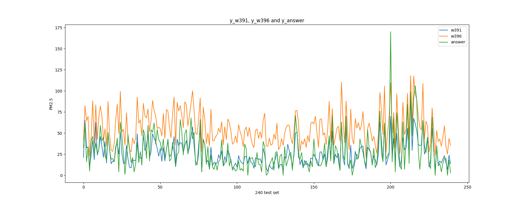
Verify data It looks like the w391 is our best output :-) for now, and the w396 is overfitting!
1 2 3 4 5 6 7 8 9 In [86 ]: lossFunction(w391,x_data_test,y_answer) Out[86 ]: 40678.24250669469 In [87 ]: lossFunction(w396,x_data_test,y_answer) Out[87 ]: 241252.78309255745 In [90 ]: lossFunction(w388,x_data_test,y_answer) Out[90 ]: 45347.799286792215
Draw the plot
1 2 3 4 5 6 7 8 9 10 11 12 13 14 15 16 17 18 19 y_w391 = np.array(y_data_w391) y_w396 = np.array(y_data_w396) y_answer = np.array(answerTestDataList[1 :]).astype(np.float ) x = range (len (y_answer)) plt.plot(x, y_w391, label="w391" ) plt.plot(x, y_w396, label="w396" ) plt.plot(x, y_answer, label="answer" ) plt.xlabel('240 test set' ) plt.ylabel('PM2.5' ) plt.title("y_w391, y_w396 and y_answer" ) plt.legend() plt.show()
The plot is as below
Start studying all other gradient descent alogrithm ref:http://ruder.io/optimizing-gradient-descent
ref:https://www.slideshare.net/SebastianRuder/optimization-for-deep-learning
ref:https://zhuanlan.zhihu.com/p/22252270
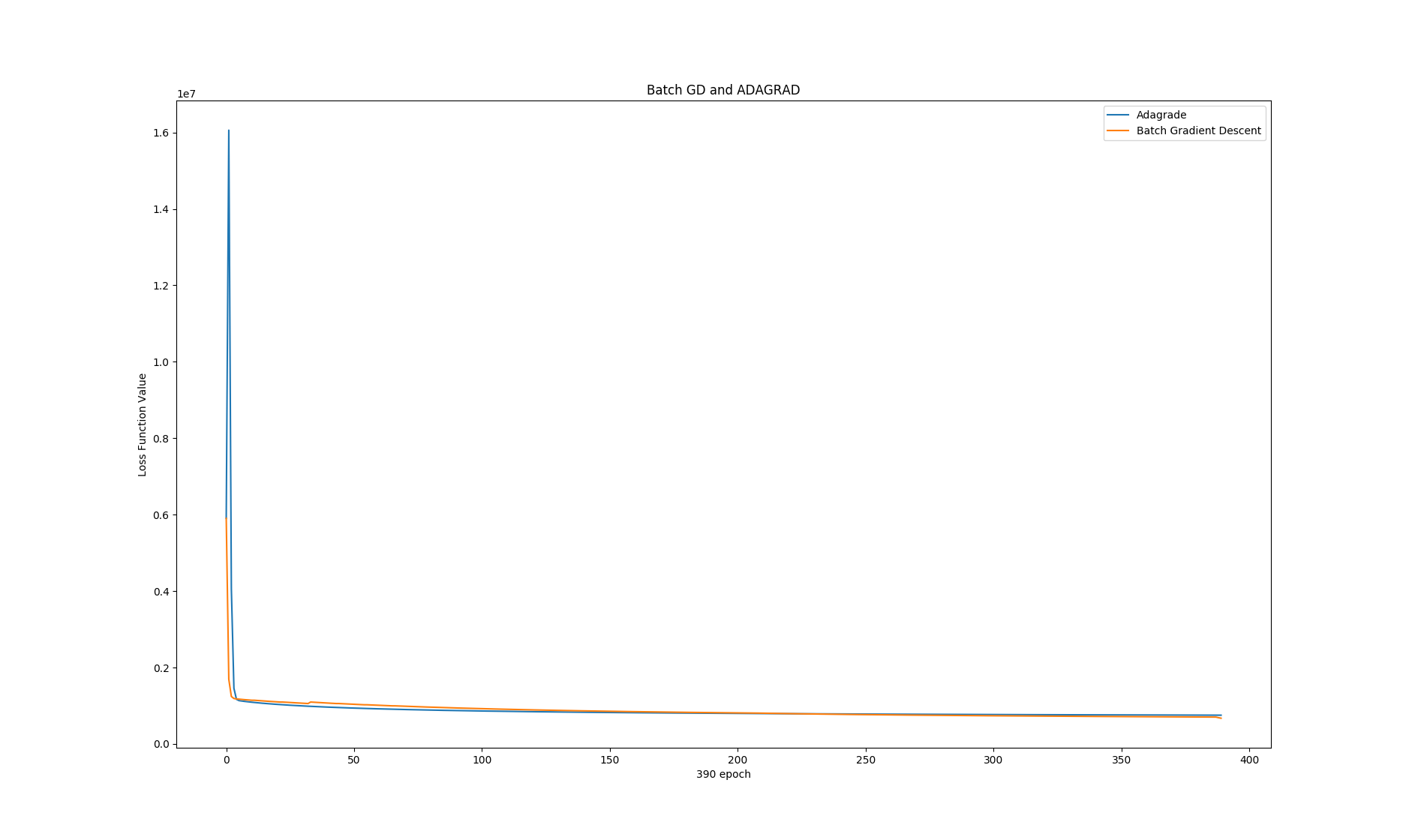
Adagrad Descent speed 1 2 3 4 5 6 7 8 9 10 11 12 13 14 15 16 17 18 19 20 21 22 23 import numpy as npimport csvimport datetimeimport matplotlibimport matplotlib.pyplot as plty_L_adagrad = np.array(L_adagrad[:391 ]) y_L_bgd = np.array(L_bgd[:391 ]) x = range (391 ) plt.plot(x, y_L_adagrad, label="Adagrade" ) plt.plot(x, y_L_bgd, label="Batch Gradient Descent" ) plt.xlabel('390 epoch' ) plt.ylabel('Loss Function Value' ) plt.title("Batch GD and ADAGRAD" ) plt.legend() plt.show()
It’s basically the same, the difference is only:
in the very begining, ADAGRAD went to crazy field, while it self corrected to normal path soon
ADAGRAD will be converging slower than BGD …
our BGD was actually human tunned one, which means ADAGRAD is easier to find themself the correct path (no need for human invention)
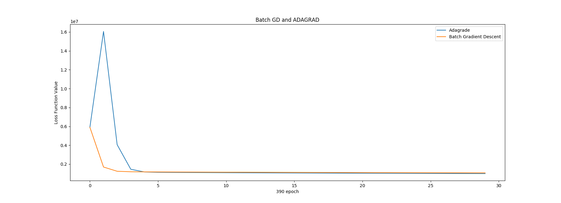
Also we could see the initial 30 epoch:
1 2 3 4 5 6 7 8 9 10 11 12 13 14 15 16 17 In [8 ]: initialN = 30 ...: y_L_adagrad = np.array(L_adagrad[:initialN]) ...: y_L_bgd = np.array(L_bgd[:initialN]) ...: x = range (initialN) ...: ...: ...: plt.plot(x, y_L_adagrad, label="Adagrade" ) ...: plt.plot(x, y_L_bgd, label="Batch Gradient Descent" ) ...: ...: plt.xlabel('390 epoch' ) ...: plt.ylabel('Loss Function Value' ) ...: ...: plt.title("Batch GD and ADAGRAD" ) ...: ...: plt.legend() ...: plt.show() ...:
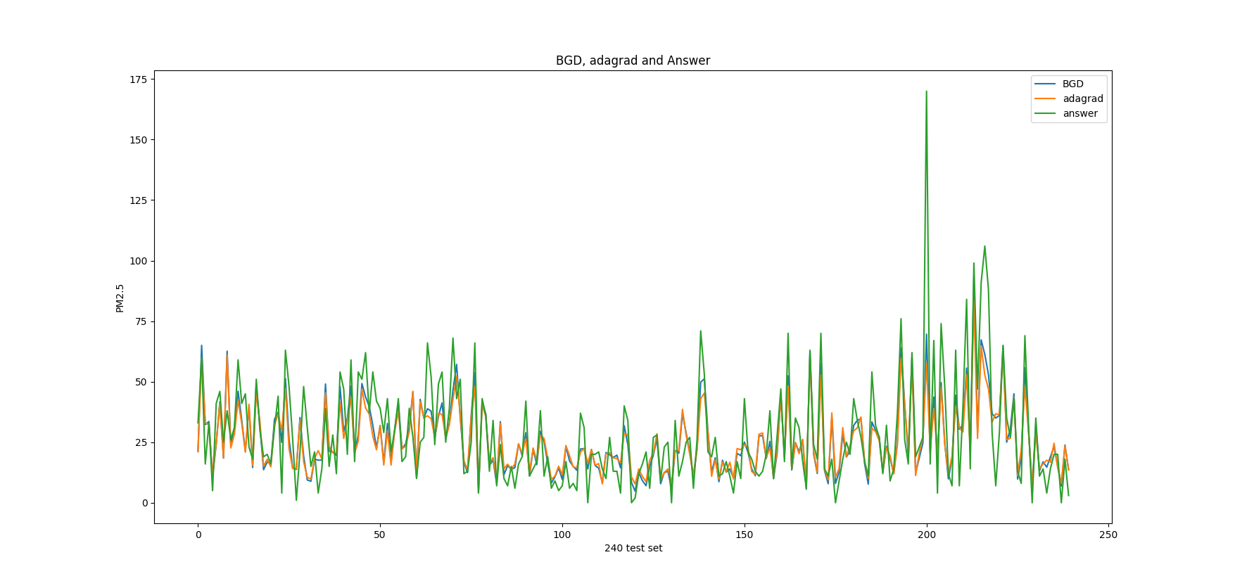
Verify the result 1 2 3 4 5 6 7 In [12 ]: lossFunction(w391,x_data_test,y_answer) Out[12 ]: 40678.24250669469 In [13 ]: lossFunction(w_adagrad,x_data_test,y_answer) Out[13 ]: 50976.42462103875
Check the prediction result figure
1 2 3 4 5 6 7 8 9 10 11 12 13 14 15 16 17 18 19 20 21 22 y_data_w391 = [y(w391,x) for x in x_data_test ] y_data_adagrad = [y(w_adagrad,x) for x in x_data_test ] y_w391 = np.array(y_data_w391) y_w_adagrad = np.array(y_data_adagrad) y_answer = np.array(answerTestDataList[1 :]).astype(np.float ) x = range (len (y_answer)) plt.plot(x, y_w391, label="BGD" ) plt.plot(x, y_w_adagrad, label="adagrad" ) plt.plot(x, y_answer, label="answer" ) plt.xlabel('240 test set' ) plt.ylabel('PM2.5' ) plt.title("BGD, adagrad and Answer" ) plt.legend() plt.show()